Marmoset Brain Connectivity Atlas

Technical White Paper: Marmoset Brain Connectivity Atlas

The marmoset brain connectivity atlas's immediate aim is to create a systematic, publicly available digital repository for data on the connections between different cortical areas, in a primate species. This initial stage takes advantage of a large collection of materials obtained over two decades of research, using fluorescent retrograde tracer injections in adult marmosets (Callithrix jacchus). Whereas several research papers have already stemmed from this material (e.g. Rosa et al. 2009; Burman et al. 2011; Reser et al. 2013; Burman et al. 2014, 2015; Majka et al. 2018), the present project represents a new initiative, towards collating these data and making them publicly available, in their entirety. We believe that sharing these materials via a digital interface will address many of the current limitations of the traditional media used for communication of neuroanatomical research, including allowing access to the entire data set (as opposed to the few sections typically illustrated in journal articles), and enabling other interpretations of the data, in light of the future evolution of knowledge about the marmoset cortex. Among other positive consequences, we hope that the availability of raw data, which can be analysed independently in different contexts, will reduce the number of animals that need to be used for research on the organization of the primate nervous systems.

As part of the present effort, we have developed techniques that allow the visualization of data (positions of injection sites, and labelled neurones) obtained in different individual monkeys, relative to the histology of the cortex. At first level, these “raw” data can be visualized in serial sections, and interpreted independently without prior assumptions regarding the identity of specific cortical areas. However, we also realize that in many cases the utility of this resource will also depend on information about the likely identity of the areas.

One of the main advantages of preserving data in digital format is the possibility of co-registering data from many different experiments into a single, navigable graphic representation (a marmoset brain template), which allows quantitative and probabilistic analyses that cannot be performed when considering data from one, or even a few injections at a time (Van Essen et al. 2012). As a step in this direction, the present resource provides the ability to visualise the data from each injection as registered into a template cortex, reconstructed from the most widely used parcellation of the marmoset brain (the Paxinos et al. 2012 atlas). This information can be accessed either as three-dimensional models of the cortex at its mid-thickness, or as bi-dimensional "unfolded" maps. The registration of each case to a template brain also allows us provide overlays for each section which provide estimates of the limits of each cortical areas.

Support

The original data collection underlying the present release was collected for a number of scientific projects, which were supported by project grants from the Australian Research Council (A09937020, DP0451206, DP0878965, DE120102883) and the National Health and Medical Research Council (237009, 384115, 384116, 491022, 545982). A list that includes papers resulting from these projects can be found here. The Australian Research Council has, in addition, provided project grants (DP110101200 and DP140101968) specifically aimed at the development of the online atlas of the marmoset brain connections, including an initial demonstration of the feasibility of this approach. Finally, the development of this resource has benefitted from the experience obtained in the NIH-funded Mouse Brain Architecture Project (RC1MH088659 and RO1MH087988). We also acknowledge internal support from both Monash University and the Cold Spring Harbor Laboratory, which was instrumental in allowing cooperative research through reciprocal visits and staff exchange. Finally, the present implementation was funded by the Australian Research Council's Centre of Excellence for Integrative Brain Function (CE140100007) and a seed grant from the International Neuroinformatics Coordinating Facility (INCF).

Why the marmoset?

Many of the techniques that provide the clearest insights on the neural basis of behaviour can only be applied to animal studies, from the production of transgenic and knockout models to physiological recordings of the electrical activity of single neurons, and high-resolution anatomical tracing. The majority of studies use rodents (Manger et al. 2008), which have provided fundamental insights on issues such as the mechanisms that regulate development of the nervous system, and synaptic physiology. However, the brains of rats, mice, and many other animal models are organized quite differently from primate brains, at the level of specific anatomical circuits. These differences include systems that are of great interest, such as those involved in the comprehension of complex visual and auditory patterns (e.g. faces and voices), and in the control of hands, and eyes. To achieve an understanding of the neural bases of these functions, neuroscientists rely on primate models (Roelfsema and Treue 2014). Although there are also obvious differences, monkey brains share several of the key anatomical circuits that differentiate us from other mammals (Orban et al. 2004).

The marmoset monkey (Callithrix spp.) is emerging as a choice animal model in systems neuroscience, which offers complementary advantages to those afforded by the more widely used macaque monkey. Marmosets are small monkeys (300-400 g adult weight), which show accelerated development in comparison with most other primates (Sawiak et al. 2018). For neuroscientists, the marmoset is important as the simplest organism that shares many of the features that make primate brains special. For example, they have well developed frontal and temporal lobes, a sophisticated visual cortex, capable of fine discriminations, multiple cortical areas involved in planning of movements, and systems involved in the interpretation of complex patterns of vocal communication (Solomon and Rosa 2014; Bakola et al. 2015; Miller et al. 2016; Wallis et al. 2017; Tani et al. 2018, among others). Yet, the topology of the marmoset brain (in particular, the cerebral cortex) is much simpler than that observed in other commonly used primates, such as the rhesus monkey. This simplifies considerably the task of registering data from different individuals to a common brain template, and makes marmosets ideal models for the optimization of the software tools that will turn a practical primate connectivity atlas into reality (Majka et al. 2016; Woodward et al. 2018). Finally, marmosets are the first primate species for which stable transgenic lines have been established (Sasaki et al. 2009), an achievement that opened the way for much-needed research on the genetic and developmental bases of primate cognition.

Tracer injections

The study of neural connections is based on substances known as neuroanatomical tracers. In a typical experiment, a surgical procedure under anaesthesia is conducted to inject few hundred nanolitres of tracer at a brain site, using a precision microsyringe. The tracer molecules diffuse in the extracellular medium, and become picked up by nearby neurons. Over a period of several days, these molecules migrate along axons, therefore revealing anatomical “bridges” that connect distant brain sites. These experiments can reveal connections that link small clusters of neurons located millimetres or centimetres away, while ignoring the overwhelming majority of intervening and adjacent cells. When considered in reference to cortical areas and thalamic nuclei, these connections tend to be very specific, and reproducible in different individuals of a same species.

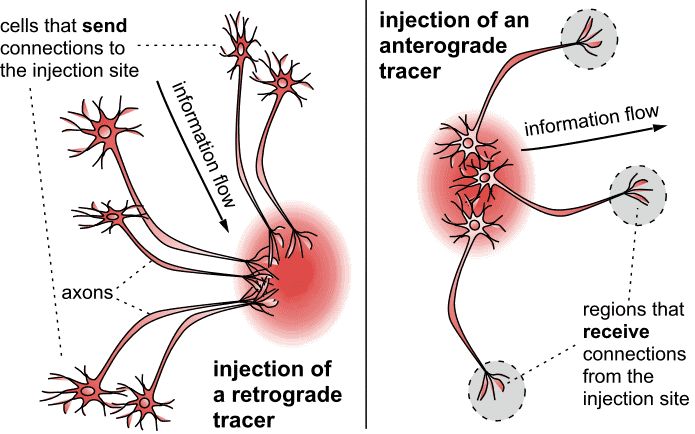
The material included in the initial release of the Marmoset Brain Connectivity Atlas is based on the use of fluorescent retrograde tracers. These are tracers that are incorporated at the synaptic terminals within the injection site, and then migrate towards the parent cell body (Figure 1, left). Retrograde tracers reveal which cells are sending information to a given neuronal population. Up to four retrograde tracers, each distinguishable by colour under a fluorescence microscope, can be used in a same animal, thus enabling the probing of connections of different brain sites in a same case. Other tracers are referred to as anterograde tracers (Figure 1, right). They are transported from the cell bodies to the synaptic terminals, thus revealing which cells are receiving information. Images showing the results of many anterograde tracing experiments in marmosets can be viewed in the Brain Architecture Project web site hosted by Cold Spring Habor laboratory http://marmoset.brainarchitecture.org, which is part of a collaborative effort towards marmoset brain mapping.

Figure 1: Tracers that are incorporated at the synaptic terminals within the injection site, and then migrate towards the parent cell body, are referred to as retrograde tracers (Left diagram). Retrograde tracers reveal which cells are sending information to a given neuronal population. Other tracers are referred to as anterograde tracers (right). They are transported from the cell bodies to the synaptic terminals, thus revealing which cells are receiving information. This image is licensed under a Creative Commons Attribution-ShareAlike 4.0 (CC-BY-SA) License. See licensing information for details.

Standardized procedures were used in creating the tracer injections, analysing, and reconstructing the data across different experiments (for details, see Majka et al. 2016). Adult marmosets (1.4-4.6 years old) of either sex were used. Metadata for each animal are provided in conjunction with each injection case. Tracers were aimed at different areas using stereotaxic coordinates obtained as part of earlier studies (for a recent review, see Paxinos et al. 2012). The exact placement of each tracer injection relative to distinct cytoarchitectural fields was determined later, following post-mortem reconstruction, both qualitatively (and histological inspection), and quantitatively (by registration to a brain template).

Six types of fluorescent tracers were used: fluororuby (FR; dextran-conjugated tetramethylrhodamine, molecular weight 10,000, 15%), fluoroemerald (FE; dextran-conjugated fluorescein, molecular weight 10,000, 15%), fast blue (FB), diamidino yellow (DY) and CTB (cholera toxin subunit B, conjugated with either Alexa 488 [CTBgr] or Alexa 594 [CTBr]). In mose cases the tracers were injected using a 1 µL microsyringe fitted with a fine glass micropipette tip. Each tracer was injected over 15–20 min, with small deposits of tracer (0.02 µL each) made at different depths. Following the last deposit (typically at a depth of 300 µm), the pipette was left in place for 3–5 min to minimize tracer reflux. In a few cases, the retrograde fluorescent tracers diamidino yellow (DY) dihydrochloride and fast blue (FB) were directly applied into the cortex as crystals, with the aid of blunt tungsten wires (Rosa et al. 2005).

Tissue processing and data analysis

After postfixation in the same medium for at least 24 h, the brains were blocked and, over the next few days, were immersed in buffered paraformaldehyde solutions containing increasing concentrations of sucrose (10%, 20%, and 30%). Frozen 40-μm sections were then obtained using a cryostat (in the vast majority of cases, coronal sections were used; a few cases were sectioned in the parasagittal plane). Every fifth section was mounted unstained on glass slides, air-dried, and coverslipped with di-n-butylphthalate-xylene mounting medium (DPX) for analysis of neurons labelled with fluorescent tracers. These sections were stored in the dark at 4 °C. Consecutive series were stained for cell bodies (using cresyl violet or Neun immunocytochemistry; Mullen et al. 1992), myelinated fibres (using a protocol adapted from Gallyas 1979), and cytochrome oxidase activity (adapted from Silverman and Tootell 1987). The protocols used in our laboratory can be downloaded from http://www.marmosetbrain.org/reference

The section viewer presented as part of the current release of the marmoset brain connectivity atlas is primarily based on Nissl stained sections. In a few cases, sections stained for the neuronal marker NeuN (Atapour et al. 2018), cytochrome oxidase, or myelin were used instead. Here, it is important to recognize that histological preparations vary in quality from case to case. Thus, our decision to provide images of all available sections necessarily meant illustrating sections that we do not consider optimal, either due to artefacts of cutting and staining, or to degradation following many years in storage. We hope that this decision to illustrate the materials “warts and all” will be seen as a positive step by our colleagues, in the sense that this will highlight aspects that deserve further investigation.

Sections were examined using Zeiss Axioplan 2 or Axioskop 40 epifluorescence microscopes. Labelled neurons were identified using ×10 or ×20 dry objectives, and their locations within the cortex and subcortical structures were mapped using a digitizing system attached to the microscope. To minimize the problem of overestimating the number of neurons due to inclusion of cytoplasmic fragments, labelled cells were accepted as valid only if a nucleus could be discerned. This was straightforward in the case of DY, as this tracer only labels the neuron's nucleus (Keizer et al. 1983). In the case of tracers that label the cytoplasm (FB, FE, and FR), the nucleus was discerned as a profile in the centre of a brightly lit, well-defined cell body, which in the vast majority of cases had an unmistakable pyramidal morphology. The entire brain was scanned in the examined series (1 in 5 sections), and every labelled neuron was plotted.

Each case in the atlas is defined by the site of a tracer injection, and by all neurons that send connections to that site (Figure 2). Within each section we encode information about the exact location of neurons that incorporated the tracer, in medial-lateral and dorsal-ventral coordinates. For example, in the case shown in Figure 2, an injection of tracer in the frontal pole of the cerebral cortex (small section, on the right) resulted in hundreds of labelled neurons in the temporal lobe and thalamus (red points indicated in the larger section, on the left).

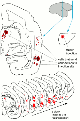
Figure 2: Illustrated are two sections through the brain of a marmoset (scale bar= 1 mm), showing a tracer injection in the frontal lobe (right) and the location of cells that send connections there (red dots on the left). Hundreds of such sections need to be combined to generate 3-d reconstructions for registration on a brain template (bottom). This image is licensed under a Creative Commons Attribution-ShareAlike 4.0 (CC-BY-SA) License. See licensing information for details.

Image Acquisition

Stained sections were scanned using Aperio Scanscope AT Turbo (Leica Biosystems) at ×20 magnification, providing a resolution of 0.50 µm/pixel. For the brains injected in the left hemisphere, the images were flipped horizontally to preserve the common format of all cases and to facilitate comparisons. We acknowledge use of the facilities and technical assistance of Monash Histology Platform, Monash University, where scanning of the sections was performed. Shortly after acquisition, the images corresponding to each section were cropped manually, rotated into a similar orientation when necessary, and saved to a separate file. All data were subsequently encoded into JPEG 2000 format, and the data were transferred into a high performance cluster to avoid loss of data due to disk failure.

Preprocessing and registration

The registration process required a series of preprocessing steps. The complete series of Nissl-stained sections from each case (i.e. one 40 μm section per 200 μm) was arranged in rostrocaudal order. The section images were downsampled to a resolution of 40 µm/pixel, and individual images were inspected for the existence of histology artefacts which were severe enough to affect the reconstruction (e.g. large folds, tears or missing parts). When necessary, “padding” was applied to correct for such artefacts, e.g. by copying the corresponding part of an adjacent section. This was routinely done at the interface between caudal and rostral blocks, where partial sections are commonly found, to preserve the overall length of the brain. The images then underwent a masking procedure during which parts of the image representing brain tissue of a single hemisphere were selected while the remaining voxels (contralateral hemisphere and the entire cerebellum) were discarded.

As detailed above, the locations of labelled neurons were encoded in a series of sections adjacent to the ones used for reconstruction (typically, the Nissl-stained series). Thus, the next preprocessing step was the alignment of the labeled cell coordinates to the histology. For this purpose we used Python scripts to extract the information and to generate Scalable Vector Graphics (SVG), resulting in a representation of the section outlines, grey/ white matter boundaries, and locations of labeled cells (for details see Majka et al. 2016). Each such drawing was manually aligned to the corresponding stained section by a simple set of translation, rotation and scaling operations. Occasionally, manual editing of the drawing was required to make it correspond correctly with the Nissl section in all locations containing labeled neurons. After the alignment the coordinates of each cell, now in the sections' coordinate system, were stored in a database.

Marmoset brain template

The objective of registering data from many different animals to a common 3-dimensional representation requires a template brain. This reference template was generated based on the electronic (PDF file) version of the Paxinos et al. (2012) marmoset brain atlas (available at: www.marmosetbrain.org/reference), which contains a complete set of cortical areas based on histological examination. This atlas uses the standard stereotaxic coordinate system based on cranial landmarks: the horizontal zero plane is defined as the plane passing through the lower margin of the orbit and the center of the external auditory meatus. The anteroposterior zero plane is defined as the plane perpendicular to the horizontal zero plane which passes the centers of the external auditory meati. The left-right zero plane is the midsagittal plane.

Delineations of cortical areas were converted into a three dimensional representation using open source 3D Brain Atlas Reconstructor software (Majka et al. 2012; http://www.3dbar.org/). The nomenclature and abbreviations followed that of the atlas. Additionally, high-resolution images of the Nissl–stained sections of the atlas specimen were downloaded (courtesy of Dr. Hironobu Tokuno; http://marmoset-brain.org), aligned with the atlas parcellation, and reconstructed into volumetric form. The resulting reconstruction preserves the exact stereotaxic coordinate system as defined in the atlas. This template is also available for download (www.marmosetbrain.org/reference).

Computational environment

The 3D reconstruction process involved multiple steps which utilized several freely available open source software packages. The Possum reconstruction framework (Majka and Wójcik, 2015; https://github.com/pmajka/poSSum) provided computational pipelines for individual sub–tasks in the reconstruction of series of two dimensional images into 3D form. Image registration was performed by the Advanced Normalization Tools (ANTS) software suite (Klein et al. 2009; Avants et al. 2011; http://picsl.upenn.edu/software/ants/). ANTS allows one to conduct rigid and affine image registration as well as deformable image warping using the Symmetric Normalisation algorithm (SyN, Avants et al. 2008) in both two- and three-dimensional images. Additional tools were used for creating, editing and composing bitmap images: Convert3D (Yushkevich et al. 2006) and ImageMagick software (http://www.imagemagick.org/). Three-dimensional visualizations were prepared using purpose–written set of Python applications utilizing the Visualization Toolkit (http://www.vtk.org/) and the Insight Toolkit (http://www.itk.org/) biomedical image processing and visualization frameworks. The computations were performed on the MASSIVE 2 cluster (https://www.massive.org.au/) under GNU/Linux operating system deployed on a dual Intel® Xeon® E5-2643 (16 × 3.30 GHz logical processors) nodes fitted with 32 GB of memory. The computational cost of the reconstruction was 200-240 CPU hours per case, depending on the number of sections.

3D reconstruction

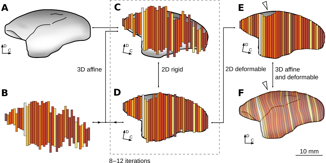
Figure 3: Reconstruction and normalization process. Note that in this illustration, for clarity, the process is represented in two dimensions. See Majka et al. 2016 for details and the technical aspects of the reconstruction process. This image is licensed under a Creative Commons Attribution-ShareAlike 4.0 (CC-BY-SA) License. See licensing information for details.

In order to co-register individual cases with the 3D template image (Figure. 3a), the set of 2D images from each case (Figure. 3b) needed to be first be reconstructed into a 3D image with realistic, anatomical shape. This was achieved by performing two types of alignments alternately (Malandain et al. 2003; Yang et al. 2012). These two steps were repeated until obtaining convergence to a reconstruction which has a faithful anatomical shape of the brain, and in which the neighboring sections are affinely aligned to one another (Figure 3c,d). The next step was to use the deformable reconstruction scheme (Adler et al. 2014; Majka and Wójcik, 2015) to account for uncorrelated, section specific distortions of the individual sections – i.e. small amounts of compression, stretching, and bending of the tissue (Figure 3e). The process of co-registration with the atlas started with the affine transformation followed by deformable warping. The latter process was driven by two similarity metrics: cross-correlation coefficient (CC, Avants et al. 2008) and the Point-Set Expectation (PSE, Avants et al. 2011) metric, which forces corresponding landmarks to overlap. Subsequently, the experimental 3D image was warped using the calculated transformations so it matches the atlas (Figure 3f).

Web Portal of viewing high resolution image with annotations

A custom web based image viewer, built around OpenLayers 3 was developed to allow fast browsing of the high resolution histology images and the corresponding parcellation and cell markings. The histology sections images are retrieved by REST-ful request and tiles of JPEG images are returned and presented to the user. The labels and markings are stored as vectors, and superimposed to the histology layer. Each type of annotation can be switched on and off at the user’s discretion.

A comprehensive search function is provided as well to provide researcher an easier way to address area of interest quickly and easily.